Computer Chronicle, One Step Further - 1. Turing Machine
Getting Started
I’ve been unpacking stories from the history of computers across several posts. The stories of the people I discovered while researching were moving. But they were not enough to understand how computers could actually be conceived and built in theoretical terms. In fact, early on in researching the history of computers, one question kept coming back to me.
So how, exactly, is a computer made and structured?
As I researched, I found at least part of an answer. So based on what I learned while preparing the computer history series, I decided to go one step deeper and write about it. About how computers could really be constructed. Unlike the more narrative historical posts, I didn’t focus as much on smooth transitions here. You can think of this as a set of posts that dig further into individual topics such as the Turing machine and the implementation of logic circuits.
I think this will read most smoothly if you already know the basics of logic gates and circuit construction, along with the kind of mathematical proofs typically covered in a second- or third-year computer science curriculum.
Of course, there are parts I’ve omitted even if they matter in real computers, especially optimization details. I’m not a core computer systems developer—in fact, I’m about as far from that domain as you can get, just an ordinary frontend developer—so there are limits to how deep I can go. If you want more detail, the books listed in the references or the original papers by the relevant researchers are good places to continue.
Enough disclaimers. In this post, I’ll look at how the "Turing machine," the theoretical foundation of the computer, came to be formulated.
Diagonalization
No one shall expel us from the paradise that Cantor has created.
David Hilbert, "Über das Unendliche", Mathematische Annalen 95, 1926
One of the major milestones leading to the idea of the computer was Cantor’s diagonal argument. It begins with thinking about infinite sets, and at first glance it seems completely unrelated to computers. But Alan Turing later used it to prove that even a universal Turing machine cannot decide certain problems. So let’s start with Cantor’s diagonal argument.
Comparing the sizes of sets and infinity
Suppose we define a "set" as a collection of objects satisfying some condition. Then how do we compare the sizes of two sets? For example, the sets and contain different elements, but both clearly have size 3. How do we express that precisely in mathematics?
We can do it by requiring that there be a one-to-one correspondence between the elements of the two sets. If every element in one set can be paired with exactly one distinct element in the other, with nothing left over, then the two sets have the same size. For example, in the sets and , we can match with , with , and with , so the two sets have the same size.
That feels intuitive. But what happens if we apply the same idea to sets with infinitely many elements? For example, consider the set of natural numbers and the set of even numbers. For any natural number , we can pair it with the even number . So there is a one-to-one correspondence between the natural numbers and the even numbers, which means the two sets have the same size. How does that feel? Is it still intuitive?
Logically it is clearly correct, but it does not feel intuitive. If the natural numbers and the even numbers have the same size, then where did all the odd numbers go? Nineteenth-century mathematicians struggled with this too. Since Euclid, it had been widely accepted that the whole is larger than a proper part. So before Cantor, many mathematicians thought the size of an infinite set was inconsistent as a concept and impossible to count meaningfully.
Cantor’s courage
Georg Cantor, a German-Russian mathematician born in 1845, began his academic career as an unpaid lecturer at the University of Halle. At the time, most mathematicians started the same way, so they needed patronage or some other source of funding made possible by notable achievements.
Around that time, the prominent mathematician Eduard Heine recognized Cantor’s talent and encouraged him to study trigonometric series—an infinite series involving trigonometric functions. That led Cantor into research on infinity.
As Cantor worked on these topics, he too ran into the counterintuitive properties of infinite sets mentioned above. The natural numbers and the even numbers are the same size? Earlier mathematicians who encountered this kind of difficulty had largely given up on handling infinity rigorously.
But Cantor chose the path that went against intuition. He argued that if two sets admit a one-to-one correspondence, then they have the same size even in the case of infinite sets, and therefore the natural numbers and the even numbers do indeed have the same size.
He then went on to prove that one-to-one correspondences also exist between the natural numbers and several other sets of numbers. There are one-to-one correspondences between the natural numbers and the integers, the rational numbers, and the algebraic numbers (numbers that are roots of algebraic equations). In other words, all of these sets have the same size. For the details and rigor of these proofs, see pages 86–87 of "오늘날 우리는 컴퓨터라 부른다" and the Schröder–Bernstein theorem.
Naturally, Cantor then turned to the set of real numbers. Is there also a one-to-one correspondence between the natural numbers and the real numbers? No—and the method Cantor used to prove this is diagonalization.
The idea of diagonalization
Then how do we know that one set is larger than another? We prove that no matter how we try to pair their elements, no one-to-one correspondence exists. For example, if we assign each element of a set to an element of a set one by one and there are still elements left over in , then is larger than .
Cantor used this to prove that the set of real numbers is larger than the set of natural numbers. To do that, he showed that the real numbers in the interval cannot be put into one-to-one correspondence with the natural numbers.
This works because itself can be put into one-to-one correspondence with the set of all real numbers . We can see this by defining a function as follows.
Now suppose there exists a function that pairs the real numbers in one-to-one with the natural numbers. Then for each , can be written as follows, where is an integer between 0 and 9.
Then we can define a real number as follows: make it differ from each in the th digit after the decimal point. There are many ways to construct such a number, but let its th digit after the decimal point be . For example, 1 becomes 2, 2 becomes 3, ..., and 9 becomes 0. If we call the th digit after the decimal point , we can write it like this.
Then for every natural number , this differs from in the th digit after the decimal point. We assumed there was a one-to-one correspondence between the natural numbers and the real numbers in , so should be equal to for some natural number —but it is not. That is a contradiction. Therefore, there is no one-to-one correspondence between the natural numbers and the real numbers in .
So the set of real numbers in the interval is larger than the set of natural numbers. And since the set of real numbers in has a one-to-one correspondence with the full set of real numbers, the set of real numbers is larger than the set of natural numbers.
There is one minor issue here. Some rational numbers can be written in two different ways. For example, and both represent the same rational number, . But this can be worked around using the fact that the set of all rational numbers also has a one-to-one correspondence with the natural numbers.
Incompleteness Theorem
Young man, in mathematics you don't understand things. You just get used to them.
Mathematicians’ dream
In the early 20th century, Hilbert and other mathematicians wanted to establish mathematics as a complete system in itself. They wanted mathematics to be expressed in a well-defined symbolic language: inside the language, each step of reasoning would be crystal clear as mathematics with meaning attached, while from outside the language it could be treated entirely as the mechanical manipulation of formulas and symbols—and still remain contradiction-free.
Here is a simple example of what it means for a system to be complete through symbol manipulation alone.
Suppose the proposition is true. And suppose I learn that is true. Then I can conclude that is also true. This does not depend on what and actually mean.
Later I may discover that meant " is even" and meant " is divisible by 2." I used the facts that is true and that to conclude that —that is, " is divisible by 2"—is true. But I did not need to know the meanings of and in order to make that inference. I could derive it purely by manipulating symbols according to rules.
Inside mathematics, these propositions carry meaning, but from outside the system we can infer new facts just by symbol manipulation. And the same would be true no matter what and meant. Even if were the axiom of choice and were the Banach–Tarski paradox (a classic counterintuitive consequence of the axiom of choice stating that one sphere can be cut into finitely many pieces and reassembled into two spheres of the same size; the precise mathematics is not important here), if we knew that was true and that , then we could still conclude that is true without understanding either concept at all.
This was the dream mathematicians pursued: to build mathematics as a system in which all of its elements could be represented in this way and manipulated without contradiction. Out of that effort came systems such as Whitehead and Russell’s Principia Mathematica and Peano arithmetic. At the 1928 International Congress of Mathematicians, Hilbert called for a proof of the completeness of Peano arithmetic.
Gödel’s proof
Two years later, in 1931, Kurt Gödel published "On Formally Undecidable Propositions of Principia Mathematica and Related Systems," resolving the issue—but not in the direction Hilbert wanted. Gödel’s paper shook Hilbert’s entire program. Setting aside that shock for a moment, let’s look at how Gödel’s proof—the step immediately preceding the Turing machine—actually works.
Gödel used somewhat different techniques, such as converting symbols into integers by exploiting the uniqueness of prime factorization rather than the decimal-style encoding I’ll use below. If needed, you can look up Gödel numbering. But since the goal here is not to follow Gödel’s original proof exactly, I’ll explain it in a more unpacked form based on Martin Davis’s "오늘날 우리는 컴퓨터라 부른다".
Attempts to build mathematics as a logical system aimed to express every element of mathematics using a finite set of symbols. They then defined rules for manipulating those symbols so that, from outside the system, mathematics could be handled entirely through those rule-based symbol manipulations.
For example, Peano Arithmetic (PA) consists of just the following 16 symbols. (Different documents may use somewhat different symbol sets, but that is not important in this context.)
Then we can prove that this system is incomplete. Let’s begin.
Most strings made from these symbols are meaningless. For example, means nothing. But some strings can be interpreted as propositions that are either true or false. For example, can be interpreted as "for every , there exists a such that ." If 1 were the identity element, this would be a proposition about the existence of inverses.
There are also strings called unary strings that define sets of natural numbers. They define a set by specifying a property of the symbol . For example, the string defining the even numbers is as follows.
Written out more explicitly, this is:
Now think carefully about the form of a unary string. If we replace the symbol it describes (in the example above, ) with a specific number, then the string becomes a proposition about that number. For example, if in the unary string above we substitute , we get , which is the proposition "2 is even."
So now, for a unary string , we can define as the proposition obtained by replacing the variable in with . For example, if is the unary string meaning "all are even," then becomes the proposition "2 is even."
Gödel’s idea is this: what matters is not what these symbols look like. As long as they preserve the same meaning, we could just as well represent them as integers. For example, could be 1, could be 2, could be 3, ..., and could be 16. From outside the system, integers are just symbols with no intrinsic meaning, so it makes no difference whether we use or 1. Of course, these numbers are just examples; representing as 2394 would work just as well.
And using this, we can construct a proposition that can never be proved within the system.
Suppose we encode these unary strings as integers. Outside the system, the encoding itself carries no meaning, but inside the system it is just a natural number. So we can order all unary strings by the size of their integer encodings.
Since every possible unary string can be encoded as an integer, the set of unary strings has a one-to-one correspondence with the natural numbers. So we can name the unary strings in increasing order of encoding size as . Here, is the unary string with the th smallest encoding.
Then for each , we can define , the proposition obtained by replacing the variable in with . Since is a unary string, is a proposition about some natural number. Then, in a way that parallels the diagonal argument—where we manipulated each to construct something new—let be the set of all such that cannot be proved within the system.
Here, "provable" means derivable from the axioms using only the rules of the system.
Regardless of how many elements it has, the set exists. That is because within PA, even sentences describing proofs of propositions can themselves be expressed using PA’s symbols, so we can define something of the form meaning "the encoding of a sentence describing a proof of the proposition encoded by is ." Then an element of would be expressed as something like .
In any case, we have now defined the set . Then surely there is a unary string that defines , and since it is also a unary string, it must be one of . Let us call that particular unary string . Then for any , means " is not provable in PA." So means " is not provable in PA."
In other words, is the proposition that says of itself that it cannot be proved. And this proposition is true. Because if we assume is false, then becomes a proposition provable in PA, and therefore true, which is a contradiction. So is certainly true from outside PA, but it is unprovable within PA itself.
Additional points
Hilbert proposed three conditions that a complete mathematical system should satisfy:
- Consistency: it must contain no contradictions. A proposition and its negation cannot both be provable.
- Completeness: every proposition must be provably either true or false within the system.
- Decidability: there must be a general procedure for proving propositions.
But Gödel’s proof above made completeness impossible. And the following argument shows that consistency is also impossible.
The proposition we constructed, , was true but unprovable in PA. Now consider its negation. For convenience, let , so the negation is . Given the original meaning of , is the proposition that it can prove itself. And since was true, the law of excluded middle tells us that is false.
So the proposition that is provable is false, and therefore is also unprovable. Since is unprovable and is also unprovable, consistency too becomes impossible.
Up to Turing’s universal machine
If the basic principle of a machine used for solving differential equations is the same as that of a machine used for issuing department store receipts, I should regard it as the most amazing coincidence I have ever encountered.
Howard Aiken1
Gödel’s incompleteness theorem, described above, denied completeness and consistency in mathematics. But decidability still remained. Is there a general algorithm that can determine the truth or falsity of any proposition after a finite number of computational steps? This question was called Hilbert’s Entscheidungsproblem, or decision problem. To prove that no such algorithm exists, Turing devised the Turing machine.
Turing first tried to express a computable algorithm in the most minimal possible form. He stripped away all unimportant details—the exact shape of the symbols used in computation, the particular structure of the machine carrying it out—and kept only the minimum elements required for computation itself. As a result, Turing arrived at the following ideas.
- At each step of a computation, only a finite number of symbols are handled.
- The action taken at each step is determined solely by the symbols currently being handled and the current state of the machine.
Turing simplified these two points even further by limiting the machine to exactly one symbol and one state at a time. Any computation that handles several things simultaneously can be replaced by one that processes them one by one over multiple steps. Combining these ideas, he created the Turing machine. He then proved that this alone is enough to represent every computable algorithm. This is called the Church–Turing thesis.
Structure of a Turing machine
A Turing machine’s computation consists of the following elements.
- A tape of infinite length and one-cell width, where each cell contains a symbol the machine can read and write
- A device that can read from and write to the tape
- The symbol currently written in the tape cell being observed
- A symbol representing the current state of the device
- The operating rules of the device (consisting of the current state, the symbol read from the tape, the symbol to write on the tape, the movement direction, and the new state)
This simple device computes by moving back and forth along the tape according to its operating rules, reading and writing the symbols on it. The exact number of tape symbols or state symbols, and what they mean, is not very important. It has been proved that adding more symbols does not change the essential power of a Turing machine.
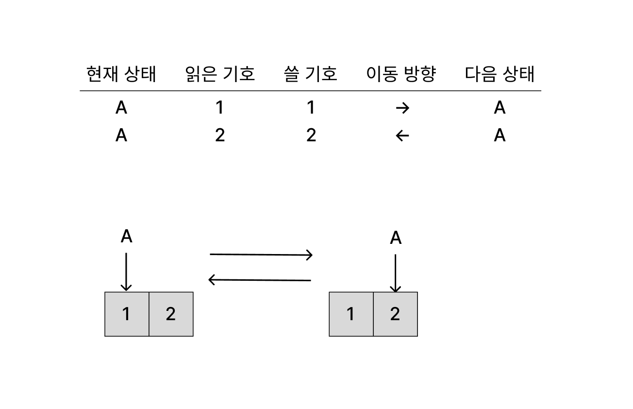
To make this more concrete, let’s build a very simple Turing machine. Suppose it works like this: when it reads 1, it writes 1 and moves right; when it reads 2, it writes 2 and moves left. Also suppose the computation starts on a tape containing 1 and 2, with the machine initially pointing at the 1. Then the machine will move back and forth across the two cells, reading and writing 1 and 2 forever. The actual tape is infinitely long, of course, but for convenience only the two relevant cells are shown in the diagram.
More complex computations—such as deciding whether a given number is even, or performing arithmetic operations—can also be implemented with a Turing machine. As mentioned above, that follows naturally from the claim that every computation can be modeled by one. But since the goal here is not to implement things directly with Turing machines, I’ll stop at this level. The books in the references include more complex examples.
Universal Turing machine
Given any computational algorithm, we can build a Turing machine that implements it. But Turing’s achievement did not stop there. He proved that a single Turing machine can simulate the computation of every Turing machine. In other words, the behavior of any Turing machine can be represented entirely by a tape and the symbols written on it, and then another Turing machine can read that representation and imitate the original machine’s behavior. After explicitly constructing such a machine, Turing called it a universal machine.
So how is this universal machine actually constructed? I’ll explain it based on Professor Kwangkeun Yi’s "컴퓨터과학이 여는 세계".
First, instead of using one tape, let us represent an arbitrary Turing machine using three tapes. Later, these will be merged into one.
On the first tape, place the tape that will be given to the Turing machine being simulated, along with an indication of the tape cell currently being pointed to. Let each tape symbol occupy two cells. We will place the symbol * to the left of a cell to indicate that it is the one currently being read.
On the second tape, store the machine’s current state. On the third tape, store the state transition table, using X as a separator. Since there are only finitely many state symbols and tape symbols, let us call them and , respectively. Then we can construct the three tapes as follows.
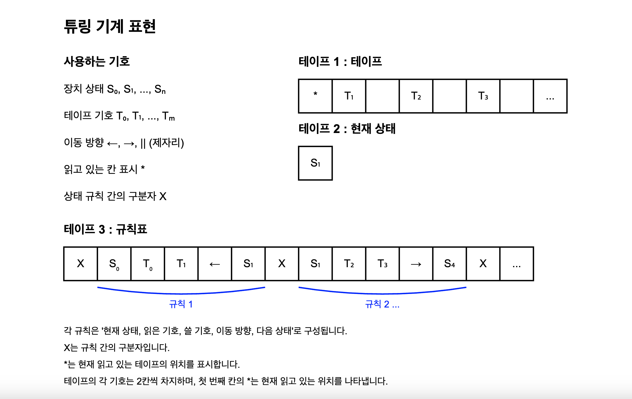
Since adding symbols does not change the power of a Turing machine, it does not matter what and are.
Now we know how to represent an arbitrary Turing machine on tapes. Then how do we construct a Turing machine that reads those tapes and simulates the behavior of the represented machine? It works like this.
- Read the current machine state from tape 2.
- Read the symbol currently being read on tape 1. This is possible by locating the
*symbol and reading the cell immediately to its right. - Search tape 3 for the rule corresponding to the current machine state and the symbol just read.
- Once the rule is found, write the appropriate tape symbol onto tape 1 as instructed, write the next machine state onto tape 2, and move the
*symbol on tape 1 left or right according to the movement direction. - Repeat steps 1 through 4.
All we have to do is express this repeated procedure as a Turing machine rule table. The rule set will be long, since it needs to search for particular symbols and copy symbols around, but in principle it is possible. This machine is then a universal Turing machine capable of simulating any Turing machine.
But one problem still remains: we used three tapes to represent an arbitrary Turing machine. However, this can be expressed using only one tape by interleaving the symbols from the three tapes.
On a single tape, write "a symbol from tape 1, a symbol from tape 2, a symbol from tape 3" repeatedly in sequence. Each symbol still occupies two cells to account for *. The tape becomes much longer, but since it is infinite, that is not an issue. In this way, any Turing machine can be represented using only a single tape.
Undecidable problems
Turing’s universal machine can represent every computable algorithm. But remember why Turing defined this universal machine in the first place: to prove that there are undecidable problems even for such a universal machine. So finally, let’s follow that argument. It too uses proof by contradiction and borrows the core idea of diagonalization.
First, suppose there exists an algorithm that can decide every proposition. Then there must of course be a Turing machine representing that algorithm; call it . Using that, we can construct a Turing machine that makes the following decision:
Given an algorithm and an input for that algorithm, does the computation eventually halt? (The Halting Problem)
Then works like this.
- Represent the Turing machine corresponding to algorithm on the tape.
- Use to decide whether the Turing machine representing the given algorithm halts on the given input.
- If the given algorithm halts, write 1 on the tape and halt. Otherwise, write 0 on the tape and halt.
For example, the Turing machine we saw earlier that moves back and forth forever on a tape containing 1 and 2 will not halt. In that case, would write 1 and halt. On the other hand, it is easy to construct a Turing machine that simply points to a cell containing 1 forever without ever moving; in that case, would write 0 and halt.
But Turing proved, using diagonalization, that no machine like can exist.
As we saw earlier, every Turing machine can be represented on a single tape. And every possible symbolic tape representation can be mapped to a natural number. Just as in the incompleteness theorem, we can do this by assigning a specific integer to each symbol. So every Turing machine and every Turing machine input can be put into correspondence with a natural number. Then, for all Turing machines and all possible inputs , could determine whether each computation eventually halts.
We can organize it as a table like this.
| 1 | 1 | 0 | 1 | ||
| 1 | 0 | 1 | 1 | ||
| 0 | 1 | 0 | 1 | ||
| 1 | 1 | 1 | 1 | ||
But then we can construct a Turing machine that behaves differently from every Turing machine in the list. Specifically, construct a Turing machine that writes 0 and halts if halts on , and writes 1 and halts if does not halt on . This is analogous to how, in the diagonal argument, we constructed a real number different from every .
That is a contradiction. A Turing machine that behaves differently from every Turing machine cannot itself exist among all Turing machines. Therefore, cannot exist. In summary, there is no algorithm that can determine the truth or falsity of every proposition.
There are many concepts derived from this, such as NP-hardness and the Busy Beaver function, which gives the maximum number of steps an -state Turing machine can take before halting—something that naturally cannot be computed by a Turing machine, since no Turing machine can decide in general whether an arbitrary Turing machine halts. If you’re interested, those are worth exploring further. But since they are not directly tied to the development of computers, I’ll leave them aside here.
Wrapping Up
So far, we’ve looked at how Turing’s universal machine can represent computable algorithms, and how undecidable problems can be constructed—problems that even such a machine cannot solve. This Turing machine became the theoretical foundation of the computer.
But implementing such a machine in a practical way is not easy. An infinitely long tape does not exist in the real world, and a machine that can read only one tape cell at a time is not very useful. The Turing machine was essentially a mathematical model.
Yet remarkably, this abstract model could be implemented as a real physical device. The foundation for that was the appearance of switches that could represent 0 and 1 as electrical signals, and Claude Shannon’s proof that logic circuits could be built from switches. As the implementation of these switches continued to improve, the computers we know became smaller and faster.
So in the next post of 'Computer Chronicle, One Step Further', I’ll probably trace the emergence and development of the switch—the device that brought the computer, once only a mathematical imagination, into the real world. And in the post after that, I hope to cover a more concrete implementation of a computer’s underlying structure using switches.
References
Knowledge typically covered in standard undergraduate computer science courses was also very helpful.
Martin Davis, translated by Park Sang-min, "오늘날 우리는 컴퓨터라 부른다", Insight
Lee Kwang-keun, "컴퓨터과학이 여는 세계: 세상을 바꾼 컴퓨터, 소프트웨어의 원천 아이디어 그리고 미래", Insight
Apostolos Doxiadis, Christos H. Papadimitriou, art by Alecos Papadatos and Annie Di Donna, translated by Jeon Dae-ho, "로지코믹스", RH Korea
Wikipedia, Church–Turing thesis
https://en.wikipedia.org/wiki/Church%E2%80%93Turing_thesis
Wikipedia, Georg Cantor
https://en.wikipedia.org/wiki/Georg_Cantor
KIAS HORIZON, Turing and the halting problem: humans, mathematics, and computers
https://horizon.kias.re.kr/19364/
Footnotes
-
Requoted from Martin Davis, translated by Park Sang-min, "오늘날 우리는 컴퓨터라 부른다", p. 212 ↩